Introduction
Last lecture:
- Model-free prediction
- Estimate the value function of an unknown MDP
This lecture:
- Model-free control
- Optimise the value function of an unknown MDP
Why we care about model-free control? So, let's see some example problems that can be modelled as MDPs:
- Helicopter, Robocup Soccer, Quake
- Portfolio management, Game of Go...
For most of these problems, either:
- MDP model is unknown, but experience can be sampled
- MDP model is known, but is too big to use, except by samples
\(\color{red}{\mbox{Model-free control}}\) can sovlve these problems.
There are two branches of model-free control:
- \(\color{red}{\mbox{On-policy}}\) learning
- "Learn on the job"
- Learn about policy \(\pi\) from experience sampled from \(\pi\)
- \(\color{red}{\mbox{Off-policy}}\) learning
- "Look over someone's shoulder"
- Learn about policy \(\pi\) from experience sampled from \(\mu\)
Table of Contents
On-Policy Monte-Carlo Control
In previous lectures, we have seen that using policy iteration to find the best policy. Today, we also use this central idea plugging in MC or TD algorithm.
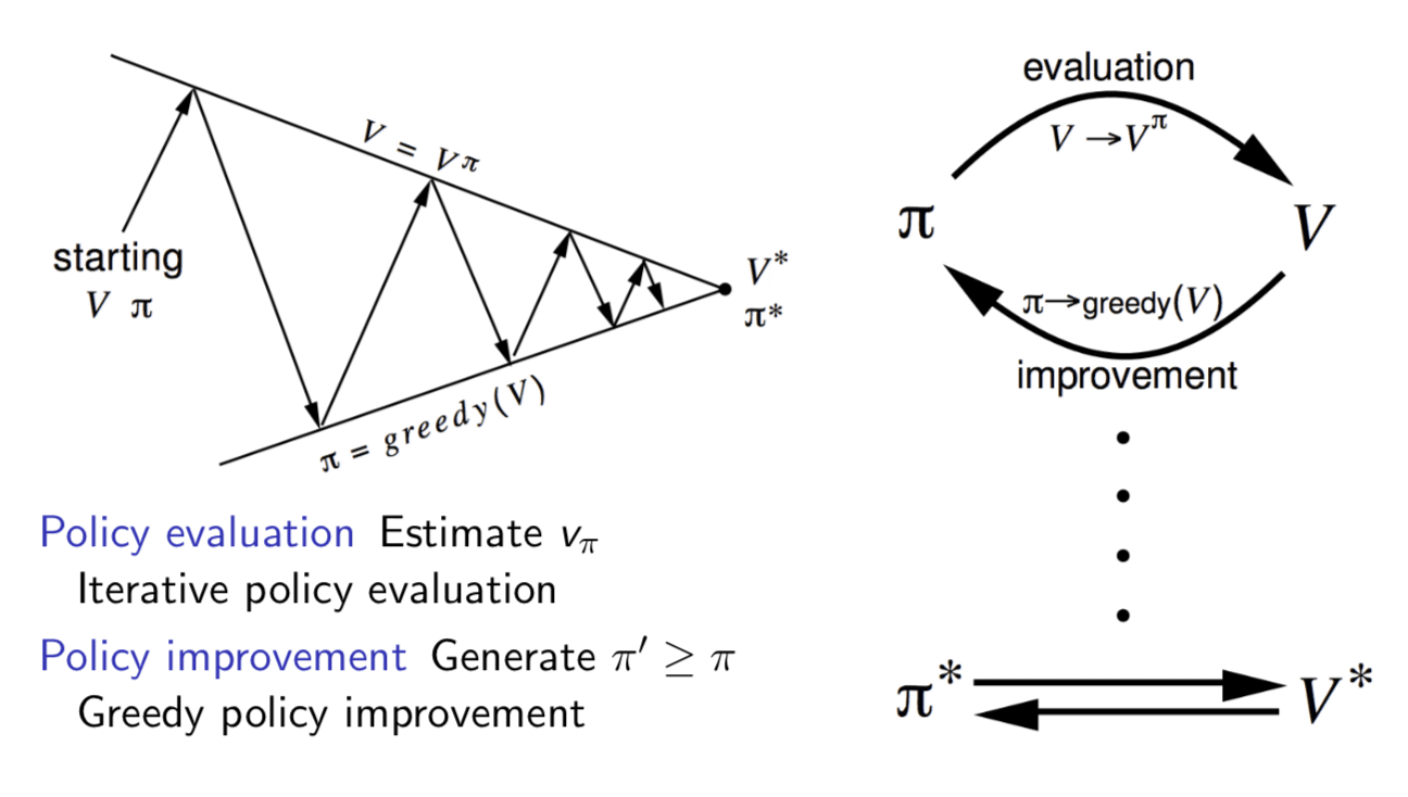
Generalised Policy Iteration With Monte-Carlo Evaluation
A simple idea is
- \(\color{Blue}{\mbox{Policy evaluation}}\): Monte-Carlo policy evaluation, \(V = v_\pi\)?
- \(\color{blue}{\mbox{Policy improvement}}\): Greedy policy improvement?
Well, this idea has two major problems:
Greedy policy improvement over \(V(s)\) requires model of MDP \[ \pi^\prime(s) = \arg\max_{a\in\mathcal{A}}\mathcal{R}^a_s+\mathcal{P}^a_{ss'}V(s') \] since, we do not know the state transition probability matrix \(\mathcal{P}\).
Exploration issue: cannot guarantee to explore all states
So, the alternative is to use action-value function \(Q\):
- Greedy policy improvement over \(Q(s, a)\) is model-free \[ \pi^\prime=\arg\max_{a\in\mathcal{A}}Q(s,a) \]
Let's replace it in the algorithm:
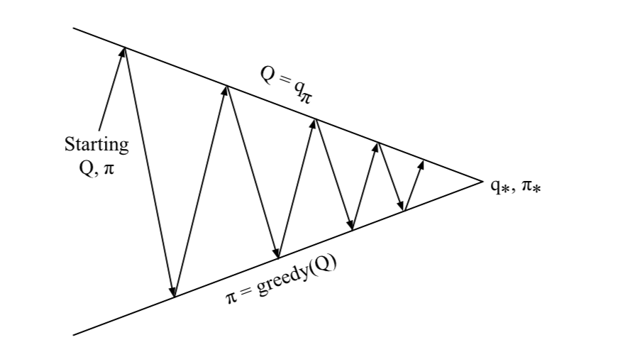
- \(\color{Blue}{\mbox{Policy evaluation}}\): Monte-Carlo policy evaluation, \(\color{red}{Q = q_\pi}\)
- \(\color{blue}{\mbox{Policy improvement}}\): Greedy policy improvement?
We still have one problems about the algorithm, which is exploration issue. Here is a example of greedy action selection:
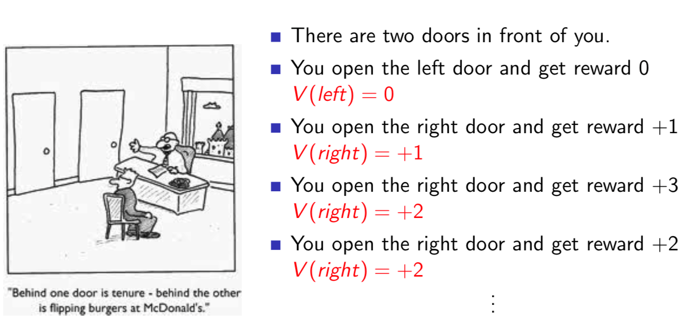
The reward of the two doors are stochastic. However, because of the greedy action selection, we always choose the right door without exploring the value of the left one.
One simple algorithm to ensure keeping exploration is \(\epsilon\)-greedy exploration.
\(\epsilon\)-Greedy Exploration
All \(m\) actions are tried with non-zero probalility,
- With probability \(1-\epsilon\) choose the greedy action
- With probability \(\epsilon\) choose an action at random
\[ \pi(a|s)=\begin{cases} \epsilon/m+1-\epsilon, & \mbox{if } a^* = \arg\max_{a\in\mathcal{A}}Q(s,a) \\ \epsilon/m, & \mbox{otherwise } \end{cases} \]
Theorem
For any \(\epsilon\)-greedy policy \(\pi\), the \(\epsilon\)-greedy policy \(\pi^\prime\) with respect to \(q_\pi\) is an improvement, \(v_{\pi^\prime}≥v_\pi(s)\).
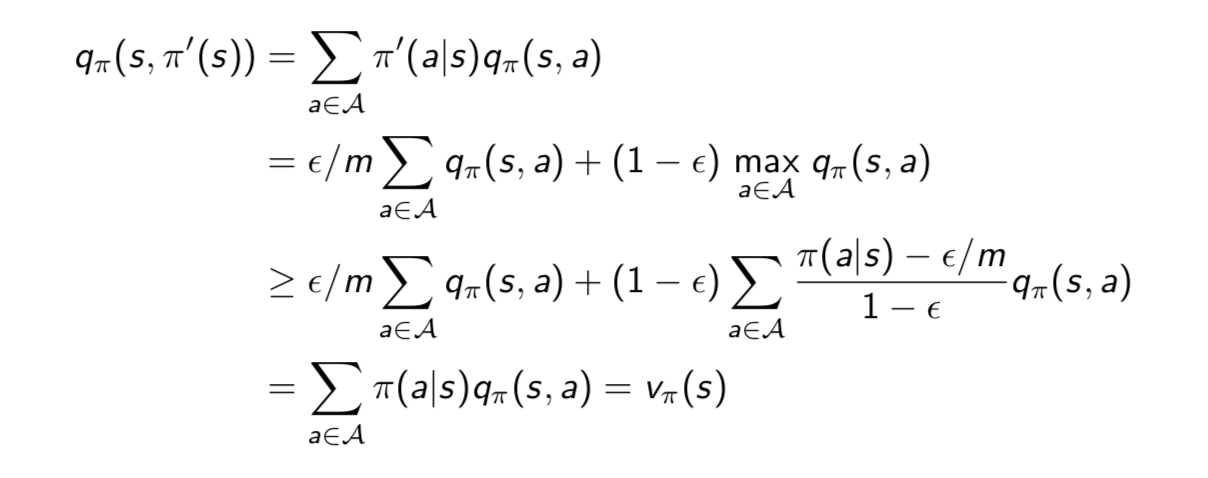
Therefore from policy improvement theorem, \(v_{\pi^\prime}(s) ≥ v_\pi(s)\).
Monte-Carlo Policy Iteration
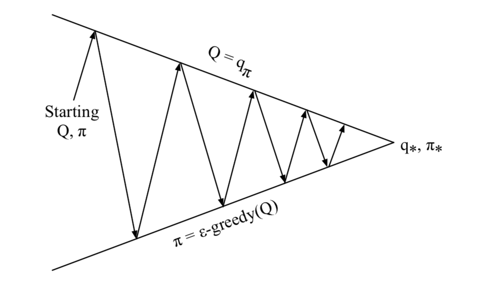
- \(\color{Blue}{\mbox{Policy evaluation}}\): Monte-Carlo policy evaluation, \(Q = q_\pi\)
- \(\color{blue}{\mbox{Policy improvement}}\): \(\color{red}{\epsilon}\)-greedy policy improvement
Monte-Carlo Control
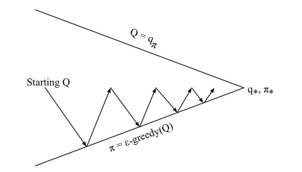
\(\color{red}{\mbox{Every episode}}\):
- \(\color{Blue}{\mbox{Policy evaluation}}\): Monte-Carlo policy evaluation, \(\color{red}{Q \approx q_\pi}\)
- \(\color{blue}{\mbox{Policy improvement}}\): \(\epsilon\)-greedy policy improvement
The method is once evaluate over an episode, immediately improve the policy. The idea is since we already have a better evaluation, why waiting to update the policy after numerous episodes. That is improving the policy right after evaluating one episode.
GLIE
Definition
Greedy in the Limit with Infinite Exploration (GLIE)
All state-action pairs are explored infinitely many times, \[ \lim_{k\rightarrow\infty}N_k(s,a)=\infty \]
The policy converges on a greedy policy, \[ \lim_{k\rightarrow\infty}\pi_k(a|s)=1(a=\arg\max_{a^\prime \in\mathcal{A}}Q_k(s, a^\prime)) \]
For example, \(\epsilon\)-greedy is GLIE if \(\epsilon\) reduces to zero at \(\epsilon_k=\frac{1}{k}\).
GLIE Monte-Carlo Control
Sample \(k\)th episode using \(\pi\): \(\{S_1, A_1, R_2, …, S_T\} \sim \pi\)
\(\color{red}{\mbox{Evaluation}}\)
- For each state \(S_t\) and action \(A_t\) in the episode, \[ \begin{array}{lcl} N(S_t, A_t) \leftarrow N(S_t, A_t)+1 \\ Q(S_t, A_t) \leftarrow Q(S_t, A_t)+\frac{1}{N(S_t, A_t)}(G_t-Q(S_t, A_t)) \end{array} \]
\(\color{red}{\mbox{Improvement}}\)
- Improve policy based on new action-value function \[ \begin{array}{lcl} \epsilon\leftarrow \frac{1}{k} \\ \pi \leftarrow \epsilon\mbox{-greedy}(Q) \end{array} \]
GLIE Monte-Carlo control converges to the optimal action-value function, \(Q(s,a) \rightarrow q_*(s,a)\).
Blackjack Example
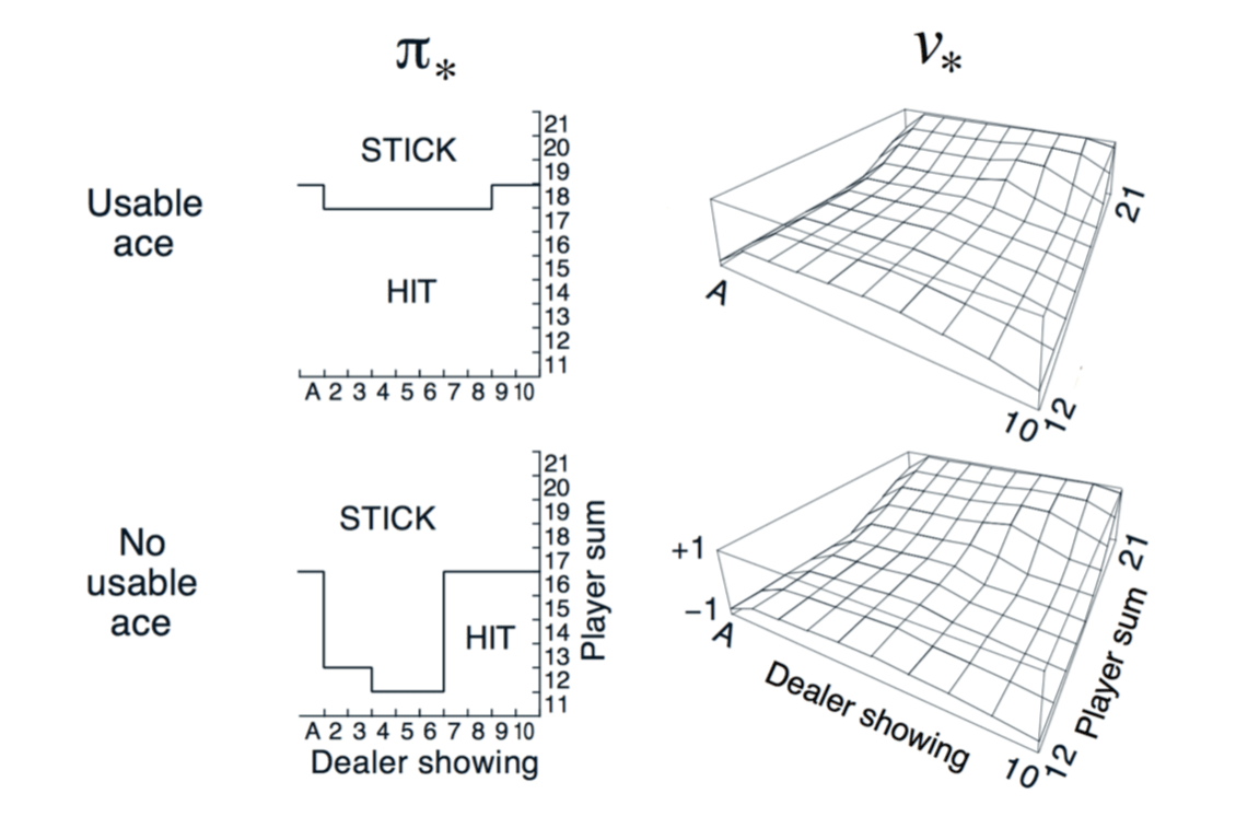
Using Monte-Carlo control, we can get the optimal policy above.
On-Policy Temporal-Difference Learning
Temporal-difference (TD) learning has several advantages over Monte-Carlo (MC):
- low variance
- Online
- Incomplete sequences
A natural idea is using TD instead of MC in our control loop:
- Apply TD to \(Q(S, A)\)
- Use \(\epsilon\)-greedy policy improvement
- Update every time-step
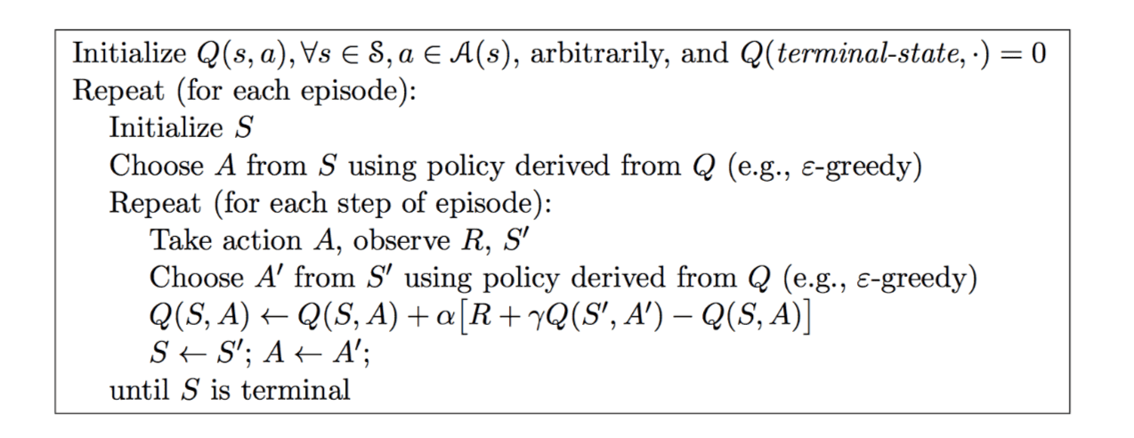
Sarsa Update
Updating action-value functions with Sarsa: \[
Q(S,A) \leftarrow Q(S, A) + \alpha(R+\gamma Q(S^\prime, A^\prime)-Q(S, A))
\]
So, the full algorithm is:
- Every \(\color{red}{\mbox{time-step}}\):
- \(\color{blue}{\mbox{Policy evaluation}}\) \(\color{red}{\mbox{Sarsa}}\), \(Q\approx q_\pi\)
- \(\color{blue}{\mbox{Policy improvement}}\) \(\epsilon\)-greedy policy improvement
Windy Gridworld Example
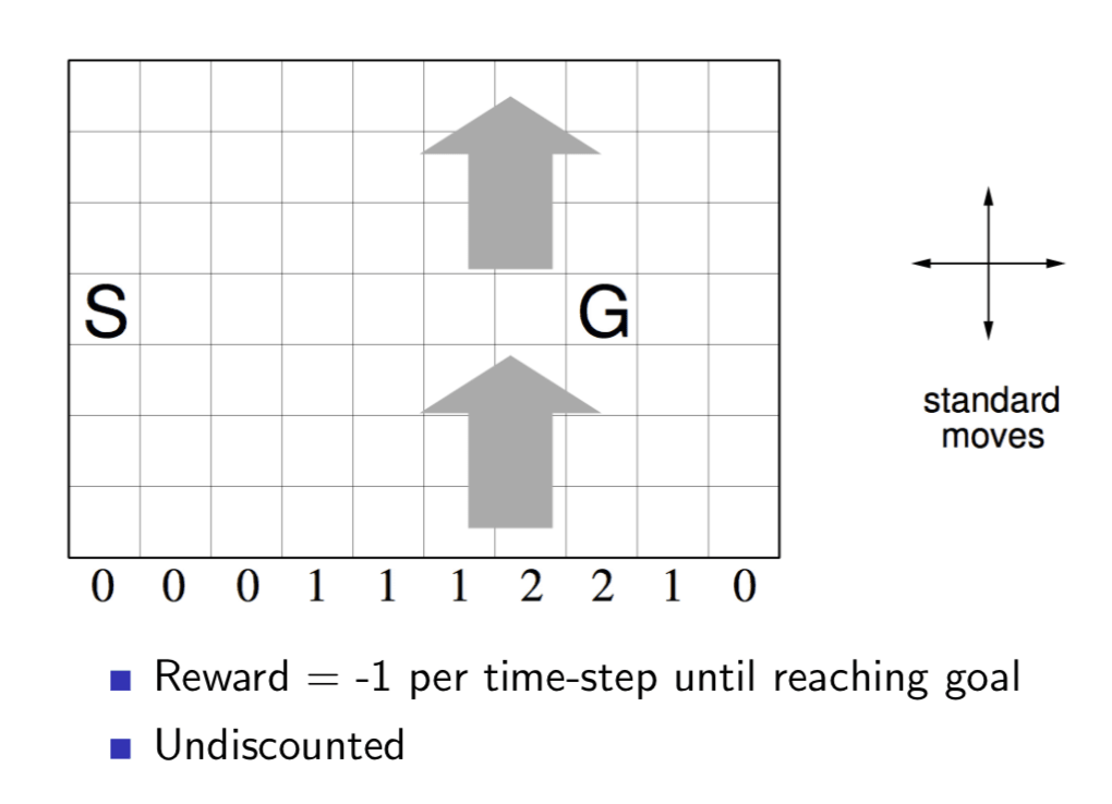
The 'S' represents start location and 'G' marks the goal. There is a number at the bottom of each column which represents the wind will blow the agent up how many grids if the agent stays at that column.
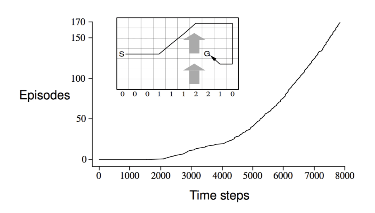
The result of apply Sarsa to the problem is
Sarsa(\(\lambda\))
n-Step Sarsa
Consider the following \(n\)-step returns for \(n=1,2,..\infty\):
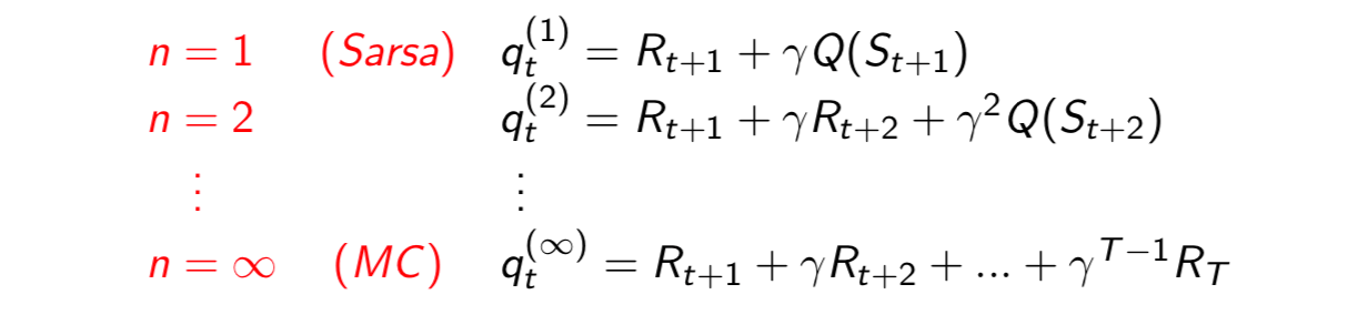
Define the \(n\)-step \(Q\)-return \[ q_t^{(n)}=R_{t+1}+\gamma R_{t+2}+...+\gamma^{n-1}R_{t+n}+\gamma^n Q(S_{t+n}) \] \(n\)-step Sarsa updates \(Q(s, a)\) towards the \(n\)-step \(Q\)-return \[ Q(S_t, A_t)\leftarrow Q(S_t, A_t)+\alpha(q_t^{(n)}-Q(S_t,A_t)) \] Forward View Sarsa(\(\lambda\))
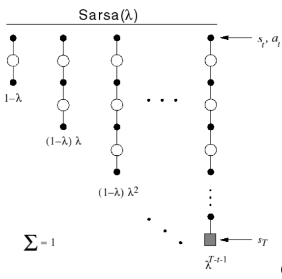
The \(q^\lambda\) return combines all \(n\)-step Q-returns \(q_t^{(n)}\) using weight \((1-\lambda)\lambda^{n-1}\): \[ q_t^\lambda = (1-\lambda)\sum^\infty_{n=1}\lambda^{n-1}q_t^{(n)} \] Forward-view Sarsa(\(\lambda\)): \[ Q(S_t, A_t)\leftarrow Q(S_t, A_t)+\alpha(q_t^\lambda-Q(S_t, A_t)) \] Backward View Sarsa(\(\lambda\))
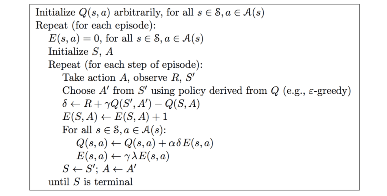
Just like TD(\(\lambda\)), we use \(\color{red}{\mbox{eligibility traces}}\) in an online algorithm, but Sarsa(\(\lambda\)) has one eligibility trace for each state-action pair: \[ E_0(s, a) = 0 \]
\[ E_t(s, a) = \gamma\lambda E_{t-1}(s,a)+1(S_t=s, A_t=a) \]
\(Q(s, a)\) is updated for every state \(s\) and action \(a\) in proportion to TD-error \(\delta_t\) and eligibility trace \(E_t(s, a)\): \[ \delta_t=R_{t+1}+\gamma Q(S_{t+1}, A_{t+1})-Q(S_t, A_t) \]
\[ Q(s, a) \leftarrow Q(s, a) +\alpha \delta_t E_t(s, a) \]
The difference between Sarsa and Sarsa(\(\lambda\)):
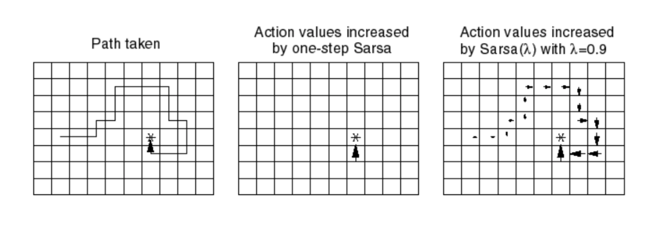
If we initial all \(Q(s, a) = 0\), then we first do a random walk and reach the goal. Using Sarsa, we can only update the Q-value of the previous state before reaching the goal since all other \(Q\) are zero. So the reward can only propagate one state. On the contrary, if we using Sarsa(\(\lambda\)), the reward can propagate from the last state to the first state with a exponential decay.
Off-Policy Learning
Evaluate target policy \(\pi(a|s)\) to compute \(v_\pi(s)\) or \(q_\pi(s, a)\) while following behaviour policy \(\mu(a|s)\) \[ \{S_1, A_1, R_2, ..., S_T\}\sim \mu \] So, why is this important? There are several reasons:
- Learn from observing hunman or other agents
- Re-use experience generated from old policies \(\pi_1, \pi_2, …, \pi_{t-1}\)
- Learn about optimal policy while following \(\color{red}{\mbox{exploratory policy}}\)
- Learn about multiple policies while following one policy
Importance Sampling
Estimate the expectation of a different distribution \[ \mathbb{E}_{X\sim P}[f(X)] = \sum P(X)f(X)=\sum Q(X)\frac{P(X)}{Q(X)}f(X)=\mathbb{E}_{X\sim Q}[\frac{P(X)}{Q(X)}f(X)] \] Off-Policy Monte-Carlo
Use returns generated from \(\mu\) to evaluate \(\pi\). Weight return \(G_t\) according to similarity between policies. Multiply importance sampling corrections along whole episode: \[ G_t^{\pi/\mu}=\frac{\pi(A_t|S_t)}{\mu(A_t|S_t)}\frac{\pi(A_{t+1}|S_{t+1})}{\mu(A_{t+1}|S_{t+1})}...\frac{\pi(A_T|S_T)}{\mu(A_T|S_T)}G_t \] Update value towards corrected return: \[ V(S_t)\leftarrow V(S_t)+\alpha (\color{red}{G_t^{\pi/\mu}}-V(S_t)) \] But it has two major problems:
- Cannot use if \(\mu\) is zero when \(\pi\) is non-zero
- Importance sampling can dramatically increase variance, so it is useless in practice
Off-Policy TD
Use TD targets generated from \(\mu\) to evaluate \(\pi\). Weight TD target \(R+\gamma V(S')\) by importance sampling. Only need a single importance sampling correction: \[ V(S_t)\leftarrow V(S_t)+\alpha \left(\color{red}{\frac{\pi(A_t|S_t)}{\mu(A_t|S_t)}(R_{t+1}+\gamma V(S_{t+1}))}-V(S_t)\right) \] This algorithm has much lower variance than Monte-Carlo importance sampling because policies only need to be similar over a single step.
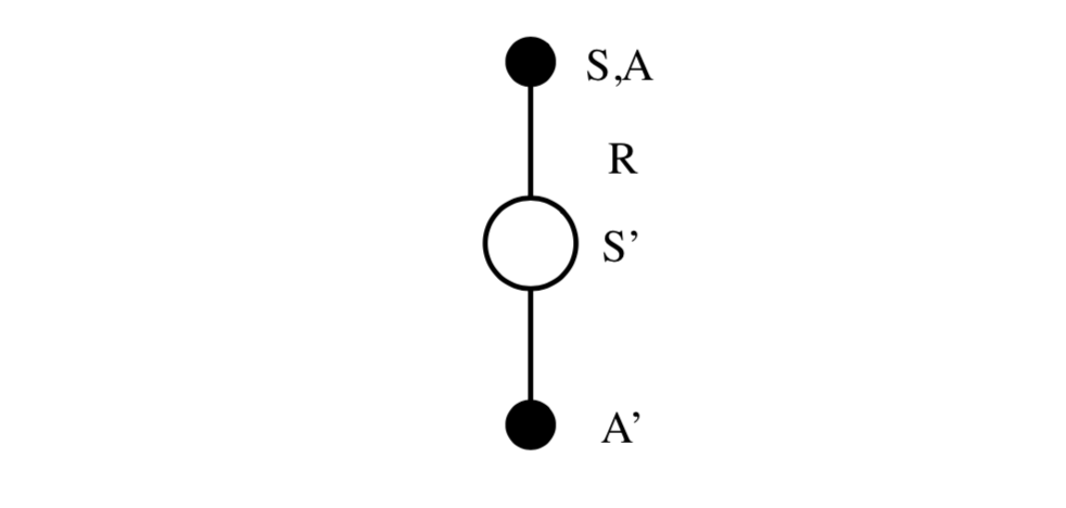
Q-Learning
We now consider off-policy learning of action-values \(Q(s, a)\). The benefit of it is no importance sampling is required.
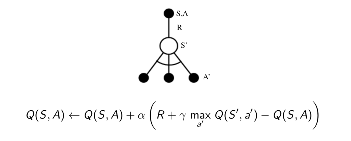
The next action is chosen using behaviour policy \(A_{t+1}\sim\mu(\cdot|S_t)\). But we consider alternative successor action \(A'\sim \pi(\cdot|S_t)\). And update \(Q(S_t, A_t)\) towards value of alternative action \[ Q(S_t, A_t) \leftarrow Q(S_t, A_t) + \alpha (R_{t+1}+\gamma Q(S_{t+1}, \color{red}{A'})-Q(S_t, A_t)) \] We now allow both behaviour and target policies to improve.
The target policy \(\pi\) is \(\color{red}{\mbox{greedy}}\) w.r.t \(Q(s, a)\): \[ \pi(S_{t+1})=\arg\max_{a'}Q(S_{t+1}, a') \] The behaviour policy \(\mu\) is e.g. \(\color{red}{\epsilon \mbox{-greedy}}\) w.r.t. \(Q(s,a)\).
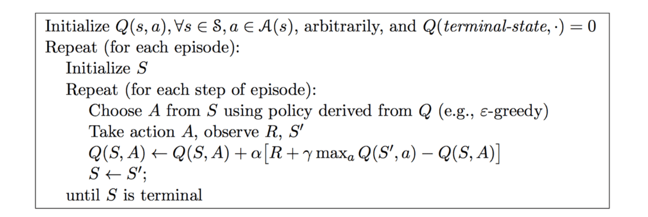
The Q-learning target then simplifies: \[ \begin{align} \mbox{Q-learning Target} &= R_{t+1}+\gamma Q(S_{t+1}, A') \\ & = R_{t+1}+\gamma Q(S_{t+1}, \arg\max_{a'}Q(S_{t+1}, a')) \\ &= R_{t+1}+\max_{a'}\gamma Q(S_{t+1}, a') \end{align} \] So the Q-learning control algorithm is
Of course, the Q-learning control still converges to the optimal action-value function, \(Q(s, a)\rightarrow q_*(s,a)\).
Summary
Relationship Between DP and TD
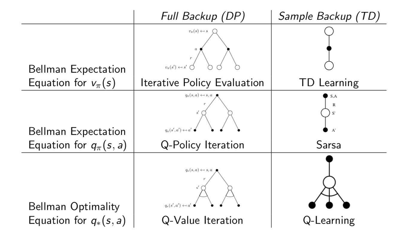
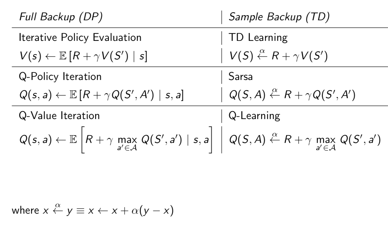
In a word, TD backup can be seen as the sample of corresponding DP backup. This lecture introduces model-free control which is optimise the value function of an unknown MDP with on-policy and off-policy methods. Next lecture will introduce function approximation which is easy to scale up and can be applied into big MDPs.